Recursive Functions of Symbolic Expressions and Their Computation by Machine, Part 1

Overview

This page contains notes on the classic paper "Recursive Functions of Symbolic Expressions and Their Computation by Machine, Part 1" by John McCarthy.

§ 2 Functions and Function Definitions

Introduces the notion of a conditional expression!

Tidbit: McCarthy proposed the addition of a cond-like expression to Algol 60, but it was rejected in favor of the English equivalent, if ... then ... else.

Review of concepts:

a. Partial Function: a function that is only defined on part of its domain.
b. Propositional Expressions and Predicates: \(T, F, \wedge, \lor, \lnot\), etc.
c. Conditional Expressions: \((p_1 \rightarrow e_1, \cdots, p_n \rightarrow e_n)\)
d. Recursive Function Definitions: \(n! = (n=0 \rightarrow 1, T \rightarrow n (n - 1)!)\)
e. Functions and Forms: Describes λ-expressions and the distinction between "forms" and "functions." The term "form" is borrowed from Church.
f. Expressions for Recursive Funcitons: \(label(a, \mathcal{E})\) allows the definition of a recursive expression by giving the expression \(\epsilon\) the label \(a\) and permitting references to \(a\) inside \(\epsilon\).

§ 3 Recursive Functions of Symbolic Expressions

Defines S-expressions, plus five (five!) elementary functions and predicates, and builds up from those five, culminating in \(apply\).

a. A class of Symbolic Expressions

Atomic symbols are S-expressions
If \(e_1\) and \(e_2\) are S-expressions, so is \((e_1 \cdot e_2)\).
\((m)\) stands for \((m \cdot NIL)\)
\((m_1, \cdots, m_n)\) stands for \((m_1 \cdot ( \cdots (m_n \cdot NIL) \cdots ))\)
\((m_1, \cdots, m_n \cdot x)\) stands for \((m_1 \cdot ( \cdots (m_n \cdot x) \cdots ))\)

b. Functions of S-expressions and the Expressions that Represent Them

Introduces M-expressions (meta-expressions)

\[ car[x] \] \[ car[cons[(A \cdot B);x]] \]

c. The Elementary S-functions and Predicates

\begin{align*} atom[X] &= T \\ atom[(X \cdot A)] &= F \\ \\ eq[X;X] &= T \\ eq[X;Y] &= F \\ eq[X;(X \cdot A)] &= \bot \\ \\ car[(e_1 \cdot e_2)] &= e_1 \\ car[X] &= \bot \\ \\ cdr[(e_1 \cdot e_2)] &= e_2 \\ cdr[X] &= \bot \\ \\ cons[e_1;e_2] &= (e_1 \cdot e_2) \end{align*}

d. Recursive S-functions

cond + recursion allows us to express all computable functions.

Here are some useful recursive functions.

\begin{align*} \text{ff}[x] = [&atom[x] \rightarrow x;T \rightarrow \text{ff}[car[x]]] \\ \\ subst [x; y; z] = [&atom[z] \rightarrow [eq[z; y] \rightarrow x; T \rightarrow z]; \\ &T \rightarrow cons [subst[x; y; car [z]]; subst[x; y; cdr [z]]]] \\ \\ equal [x; y] = [&atom[x] \wedge atom[y] \wedge eq[x; y]] \lor \\ [&\lnot atom[x] \wedge \lnot atom[y] \wedge equal[car[x]; car[y]] \wedge equal[cdr[x]; cdr[y]]] \\ \\ null[x] = &atom[x] \wedge eq[x;NIL] \end{align*}

And some functions on lists.

\begin{align*} append[x; y] = [&null[x] \rightarrow y; T \rightarrow cons[car[x]; append[cdr[x]; y]]] \\ \\ among[x; y] = &\lnot null[y] \wedge [equal[x; car[y]] \lor among[x; cdr[y]]] \\ \\ pair[x; y] = [&null[x] \wedge null[y] \rightarrow NIL; \\ &\lnot atom[x] \wedge \lnot atom[y] \rightarrow cons[list[car[x]; car[y]]; pair[cdr[x]; cdr[y]]] \\ \\ assoc[x; y] = &eq[caar[y]; x] \rightarrow cadar[y];T \rightarrow assoc[x; cdr[y]]] \\ \\ sub2[x; z] = [&null[x] \rightarrow z; eq[caar[x]; z] \rightarrow cadar[x];T \rightarrow sub2[cdr[x]; z]] \\ \\ sublis[x; y] = [&atom[y] \rightarrow sub2[x; y];T \rightarrow cons[sublis[x; car[y]]; sublis[x; cdr[y]]] \end{align*}

e. Representation of S-Functions by S-Expressions

How to translate M-expressions into S-expressions.

"The translation is determined by the following rules in which we denote the translation of an M-expression \(\mathcal{E}\) by \(\mathcal{E}^{\ast}\)"

If \(\mathcal{E}\) is an S-expression, \(\mathcal{E}^{\ast}\) is \((QUOTE, \mathcal{E})\).
Symbols get converted to uppercase. \(car^{\ast} \mapsto CAR, subst^{\ast} \mapsto SUBST\)
\(f[e_1; \cdots; e_n] \mapsto (f^{\ast}, e_1^{\ast}, \cdots, e_n^{\ast})\). Thus, \(cons[car[x]; cdr[x]]^{\ast} \mapsto (CONS, (CAR, X), (CDR, X))\).
\(\{[p_1 \rightarrow e_1; \cdots; p_n \rightarrow e_n]\}^{\ast} \mapsto (COND, (p_1^{\ast},e_1^{\ast}), \cdots, (p_n^{\ast},e_n^{\ast}))\)
\(\{\lambda[[x_1;\cdots;x_n];\mathcal{E}]\}^{\ast} \mapsto (LAMBDA, (x_1^{\ast},\cdots,x_n^{\ast}), \mathcal{E}^{\ast})\)
\(\{label[a;\mathcal{E}]\}^{\ast} \mapsto (LABEL, a^{\ast}, \mathcal{E}^{\ast})\)

f. The Universal S-Funciton, \(apply\)

Behold!

The S-function apply is defined by

\[ apply[f; args] = eval[cons[f; appq[args]];NIL], \]

where

\[ appq[m] = [null[m] \rightarrow NIL;T \rightarrow cons[list[QUOTE; car[m]]; appq[cdr[m]]]] \]

and¹

\begin{equation*} \begin{split} eval[&e; a] = [ \\ &atom[e] \rightarrow assoc[e; a]; \\ &atom[car[e]] \rightarrow [ \\ & \quad \quad eq[car[e]; QUOTE] \rightarrow cadr[e]; \\ & \quad \quad eq[car[e]; ATOM] \rightarrow atom[eval[cadr[e]; a]]; \\ & \quad \quad eq[car[e]; EQ] \rightarrow [eval[cadr[e]; a] = eval[caddr[e]; a]]; \\ & \quad \quad eq[car[e]; COND] \rightarrow evcon[cdr[e]; a]; \\ & \quad \quad eq[car[e]; CAR] \rightarrow car[eval[cadr[e]; a]]; \\ & \quad \quad eq[car[e]; CDR] \rightarrow cdr[eval[cadr[e]; a]]; \\ & \quad \quad eq[car[e]; CONS] \rightarrow cons[eval[cadr[e]; a]; eval[caddr[e]; a]]; \\ & \quad \quad T \rightarrow eval[cons[assoc[car[e]; a]; cdr[e]]; a]]; \\ &eq[caar[e]; LABEL] \rightarrow eval[cons[caddar[e]; cdr[e]]; cons[list[cadar[e]; car[e]]; a]; \\ &eq[caar[e]; LAMBDA] \rightarrow eval[caddar[e]; append[pair[cadar[e]; evlis[cdr[e]; a]; a]]] \end{split} \end{equation*}

and

\[ evcon[c; a] = [eval[caar[c]; a] \rightarrow eval[cadar[c]; a];T \rightarrow evcon[cdr[c]; a]] \]

and

\[ evlis[m; a] = [null[m] \rightarrow NIL;T \rightarrow cons[eval[car[m]; a]; evlis[cdr[m]; a]]] \]

g. Functions with Functions as Arguments

\[ maplist[x; f] = [null[x] \rightarrow NIL;T \rightarrow cons[f[x];maplist[cdr[x]; f]]] \]

\[ search[x; p; f; u] = [null[x] \rightarrow u; p[x] \rightarrow f[x];T \rightarrow search[cdr[x]; p; f; u] \]

§ 4 The LISP Programming System

a. Representation of S-Functions by List Structure

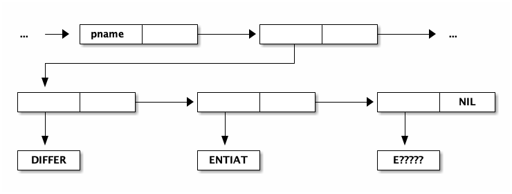
Introduces the boxes & arrows notation for cons cells. Substructure can be shared, but cycles are not allowed. Symbols are represented as "association lists" (property lists in modern usage) where the car is a magic constant indicating the cons is a symbol.

b. Association Lists (P-lists)

P-list may contain:

print name
symbol value (number, sexp, function)

A P-list is not a sexp. For example, the print name of a symbol is represented as follows:

c. Free-Storage List

The system starts with ~15k words on the free list.
Some fixed register contains the start address of the free list.
To cons, pop words from the head of the free list.
gc works as follows (standard mark & sweep):
- a fixed set of base registers serve as gc roots.
- don't collect until out of blocks on the free-list
- when out of memory:
  - start from roots and mark all reachable words by negating the signs (essentially, first bit is a mark bit).
  - if you find reg with sign, assume it's already been visited.
  - sweep through the heap and put any un-marked words back on the free list and revert mark bits.

McCarthy notes that a gc cycle took several seconds to run!

d. Elementary S-Functions in the Computer

S-expressions are passed to / returned from functions as pointers to words.

atom: Test car for magic value, return symbol \(T\) or \(F\), unless appearing in \(cond\), in which case transfer control directly without generating \(T\) or \(F\).
eq: pointer compare on address fields. As above, generate \(T\) or \(F\) or \(cond\) transfer.
car: access "contents of address register".
cdr: access "contents of decrement register".
cons: \(cons[x;y]\) returns the location of a word with \(x\) in the car and \(y\) in the cdr. Doesn't search for existing cons, just pulls a new one from the free list. \(cons\) is responsible for kicking off a gc cycle when out of memory.

e. Representation of S-Functions by Programs

SAVE/UNSAVE: push/pop registers from/onto the "public pushdown list" (a.k.a. stack). Only used for recursive functions?

f. Status of the LISP Programming System (Feb. 1960)

Can define S-Functions via S-expressions. Can call user-defined and builtin functions.
Can compute values of S-Functions.
Can read/print S-expressions.
Includes some error diagnostics and selective tracing.
May compile selected S-Functions.
Allows assignment and go to, ala ALGOL.
Floating point possible, but slow.
LISP 1.5 manual coming soon!

§ 5 Another Formalism for Functions of S-expressions

So-called, L-expressions (Linear LISP).

Permit a finite list of chars
Any string of permitted chars is an L-expr, including the null string, denoted \(\Lambda\).

There are three functions:

\(first[x]\) is the first char of \(x\). \(first[\Lambda] = \bot\).
\(rest[x]\) is the string of chars remaining after first is deleted. \(rest[\Lambda] = \bot\).
\(combine[x;y]\) is the string formed by prefixing \(x\) to \(y\).

There are also three predicates:

\(char[x] = T \iff x\) is a single char.
\(null[x] = T \iff x = \Lambda\)
\(x = y\) is defined for \(x\) and \(y\) characters.

§ 6 Flowcharts and Recursion

Presents an interesting scheme for converting program blocks + branches into recursive functions. Considers each program block as a function \(f\) from the current program state \(\xi\) to a new state \(\xi'\), i.e. \(\xi' = f[\xi]\). Blocks can be combined by decision elements, represent with the symbol \(\pi\).

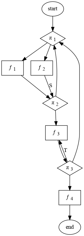
We give as an example the flowcart of figure 5. Let us describe the function \(r[\xi]\) that gives the transformation of the vector \(\xi\) between entrance and exit of the whole block. We shall define it in conjunction with the functions \(s(\xi)\), and \(t[\xi]\), which give the transformations that \(\xi\) undergoes between the points \(S\) and \(T\), respectively, and the exit. We have

\begin{align*} r[\xi] &= [\pi_1[\xi] \rightarrow S[f_1[\xi]];T \rightarrow S[f_2[\xi]]] \\ S[\xi] &= [\pi_2[\xi] \rightarrow r[\xi];T \rightarrow t[f_3[\xi]]] \\ t[\xi] &= [\pi_{3_1}[\xi] \rightarrow f_4[\xi]; \pi_{3_2}[\xi] \rightarrow r[\xi];T \rightarrow t[f_3[\xi]]] \end{align*}

Footnotes:

I corrected a couple of minor errors in \(eval\), namely a missplaced bracket in the \(LABEL\) clause and an extraneous \(evlis\) that caused double-evaluation of function arguments when calling a procedure bound to a variable.